PID controller step input characteristics

In this post I will show some theoretical analysis of the PID controller that we have designed in my previous post. After going through this post one will be able to under stand how to derived transfer function of a PID controller, what are the different characteristics of step input response and how are they defined. Finally we will use the data that we have collected in previous postduring the experiment to simulate a PID controller and analyze its step response.

Transfer function of a PID controller

A PID controller block, takes the error signal as input and generates control output signal. In time domain if we define control input as \(u(t)\) and error signal as \(e(t)\), then based on the definition of PID controller, we write

\[u(t) = K_Pe(t) + K_I\int e(t) + K_D \dot{e}(t)\]

Taking the Laplace transform we get,

\[U(s) = (K_P + K_I/s + K_Ds)E(s)\]

Therefore transfer function of the PID block is obtained as,

\[T(s) = \frac{U(s)}{E(s)} = K_P + \frac{K_I}{s} + K_Ds\]

In some applications, it is beneficial to express \(K_I = K_P/T_i\) and \(K_D = K_PT_d\), where \(T_i\) and \(T_d\) are integration and derivative time horizons. This is exactly what we did in PID experiment post to derive the transfer function. In this case, the transfer function of PID controller block would look like as,

\[T(s) = \frac{U(s)}{E(s)} = K_P(1 + \frac{1}{T_is} + T_ds)\]

Characteristic of Step Response

There are three main characteristics of the step response.

1. Rise time
2. Settling time
3. Percentage of Overshoot

Rise time \((T_r)\): The time that the response signal would take to reach to 90% from 10% of the steady-state response.

Settling time \((T_s)\): The time that the response signal would take to settle within 2% error relative to the steady-state response.

Percentage of Overshoot: Percentage difference between the maximum peak of the response and steady state response, relative to the steady state response.

Simulated response of turntable

We are now ready to simulate the response of the same PID turn-table experiment for a unit step input. After that we will report the step response characteristics for the simulated system.

From out experiment we found that, the PID controller parameters are \(K_P = 2, T_d = 5e-4 min, T_i = 5e-5 min\). We will be using these paameters to implement the controller. The other system parameters are given in PID turn-table experiment post and will be used them in SI unit form in the simulation.

The python script for simulating the system response with PID controller is given below.

from mpmath import *
import matplotlib.pyplot as plt

def fp(p):
    # Define the given parameters
    Ra = 11.5
    Kb = 12*60/1000                      # convert to V/RPS
    Kt = 12*60/1000                      # convert to V/RPS
    Km = 16.2*0.02835*9.81*0.0254        # convert FPS to SI unit
    J = 2.5*0.02835*9.81*(0.0254**2)     # convert FPS to SI unit
    b = 0
    Kc = 1
    Ti = 0.0005*60                       # convert minute to second
    Td = 0.00005*60                      # convert minute to second

    G = Km/(Ra*(J*p+b)+Kb*Km)            # TF of load
    Gc = Kc*(1 + 1/(Ti*p) + Td*p)        # TF of PID controller
    # Gc = Kc*(1 + Td*p)
    # Gc = Kc
    return Gc*G/(p*(1+Kt*Gc*G))          # TF of the whole system
    
def step_info(resp, t, resp_final):
	# Find the index for 10% and 90% of total response
	tol = 1e-1
	tl_ind, th_ind, ts_ind, tp = 0, 0, 0, 0
	vl, vh, vs_l, vs_h = 0.10*resp_final, 0.90*resp_final, 0.98*resp_final, 1.02*resp_final
	peak_val = 0 
	for ind, val in enumerate(resp):
		# print(ind, val, abs(val-vs), abs(val-resp_final))
		if abs(val-vl) < tol:
			tl_ind = ind
		if abs(val-vh) < tol:
			th_ind = ind
		if ts_ind != 0:
			if vs_l > val or vs_h < val:
				ts_ind = 0
		if vs_l < val and vs_h > val and ts_ind == 0:
			ts_ind = ind
		if val > peak_val:
			peak_val = val
	print("Rise time: %1.3f sec"%(t[th_ind]-t[tl_ind]))
	print("Settling time: %1.3f sec"%t[ts_ind])
	print("Overshoot: %2.3f percent"%((peak_val-resp_final)*100/resp_final))
	return tl_ind, th_ind, ts_ind

mp.dps = 5; mp.pretty = True

# Set point
set_pt = 1000/12

# Generate time vector
tm = [0.0001*tm for tm in range(1, 5000)]

# Multiply the output with 60 to convert RPS to RPM
omega_res = [60*invertlaplace(fp,tt,method='talbot') for tt in tm] # RPM

# Call step_info
stepInfo = step_info(omega_res, tm, set_pt)

plt.plot(tm, omega_res)
plt.plot([tm[stepInfo[0]], tm[stepInfo[0]]], [0, omega_res[stepInfo[0]]], "C1")
plt.plot([tm[stepInfo[1]], tm[stepInfo[1]]], [0, omega_res[stepInfo[1]]], "C1")
plt.plot([tm[stepInfo[2]], tm[stepInfo[2]]], [0, omega_res[stepInfo[2]]], "C2")
print(omega_res[stepInfo[1]]/2)
plt.text(tm[stepInfo[1]]/2, omega_res[stepInfo[1]]/2, "rise time")
plt.text(tm[stepInfo[2]], omega_res[stepInfo[2]]/2, "setteling time")
plt.xlabel("time [s]")
plt.ylabel(r"$\omega$(t) [RPM]")
plt.title("Step response for PID controller")
plt.grid()
plt.show()

The simulated response of the turntable with PID controller is found after running the above script is shown below.

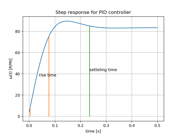
The rise time, settling time and percent of overshoot values are found to be,

Rise time: 0.073 sec
Settling time: 0.235 sec
Overshoot: 7.474 %

LABVIEW application

The figure below shows the basic LABVIEW program that can be used to acquire and send signal to the system for the DAQ connections as per the post on PID experiment post.

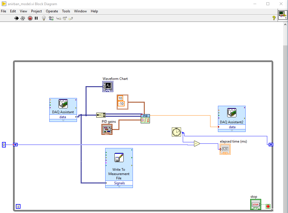
I only used a few number of code blocks to achieve the above and they are

• DAQ Assistant (1 input and 1 output)
• Waveform Chart
• Write to Measurement File
• PID
• Split Signal
• While Loop with Button
• While Shift
• Numeric
• Cluster
• Create Control
• Comparison
• Elapsed Time