Robotics Projects
Monte-Carlo-Localization for Tracking a Moving Object
The repository can be found here.
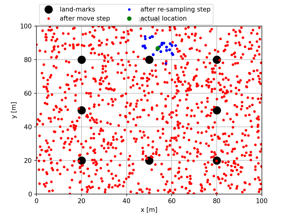
In the above figure (generated by running main_one_file.py), the actual location of the car is visualized as the green circle where as the distribution of the posteriors are shown in blue particles and prior beliefs are shown in red particles. Notice that initially, we were completely uncertain about the actual location of the car and that is why particles are distributed everywhere in the world. However, after a few iterations most of the particles were clustered around the actual location of the car with a small error covariance.
The particle filter implementation here has the following key steps,
-
Initialize a number of particles in the environment by uniformly sampling (uniform random sampling) the range of X and Y coordinates. At this time we have no information of the actual location of the car since we have no sensed data.
-
In order to simulate the actual behavior of the car, we create a
fake_robotobject which moves around the environment and sends sensed data. -
Next for each move that the fake robot makes and gives new measurement of the environment, we perform a two stage manipulation on each particle. Firstly, we move each particle with equal amount and let them have their own measurement of the environment. Secondly, based on how close the measurement of each particle matches with the actual cars measurement we assign importance weight to each particle. Finally carry out resampling of the particles such that particles with higher weights have many copies and lower weights has less number of copies.
There are many resampling strategies out there, however here we have followed the one explained here.
Below we make a comparison of the advantage of using Particle Filter over Extended Kalman Filter.
- Particle filter can capture arbitrary distribution of the prior and the posterior. But EKF can only represent these distributions as Gaussian distribution.
- In EKF, nonlinearity in observer and measurement model is approximated as linear models. Unlike EKF, the Particle Filter does not need the linearization of the nonlinear observer and measurement models.
- Particle Filter is easy to understand and implement. EKF requires to understand involved mathematical treatment.
- However particle filter provides a discrete distribution of the prior and posterior. But EKF provides continuous distribution of those distributions.
- In terms of computational complexity, particle filter is worse than EKF.
- Overall particle filter has gained more popularity because of its simplicity of implementation and its power to capture multimodal distribution of the prior and posterior with no need of linearization (computing the Jacobians) of the nonlinear observer and measurement models.
Robust Localization Fusing LASER and RADAR Data
The repository can be found here.
In this project, location of a moving car is localized fusing RADAR and LASER data. In reality, the radar and laser sensor are fixed on top of the moving car so that we get updated measurement from these sensors as the car moves around. In this project the sensor data are given in a text file, located in data/obj_pose-laser-radar-synthetic-input.txt. The data looks as follows,
L	3.122427e-01	5.803398e-01	1477010443000000	6.000000e-01	6.000000e-01	5.199937e+00	0	0	6.911322e-03
R	1.014892e+00	5.543292e-01	4.892807e+00	1477010443050000	8.599968e-01	6.000449e-01	5.199747e+00	1.796856e-03	3.455661e-04	1.382155e-02
The letter L describes all the following values in that row pertaining to the LASER data whereas R stands for RADAR. The data are labeled as,
L meas_px meas_py tm gt_px gt_py gt_vx gt_vy
R meas_rho meas_phi meas_rho_dot timestamp gt_px gt_py gt_vx gt_vy
The key steps in achieving robust localization fusing sensor data are as follows,
- Get the measurement information, either from RADAR or LASER by reading one row at a time from the data file.
- Now we will know the measured location of the car along with the time-step value.
- Assuming the observer model of the car is linear, we predict car location with respect to time-step value.
- The measurement update is done using Kalman Filter (KF) or Extended Kalman Filter (EKF) depending on the current measurement is from LASER or RADAR. Since the measurement equation of the RADAR is non-linear we need to use EKF for the update step.
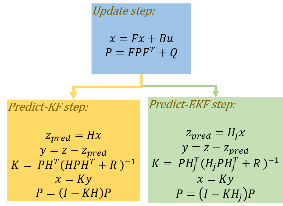
The relevant equations used for prediction and steps are show in the figure below,
 .
.
The matrix H in the update-KF step indicates linear measurement model (LASER) whereas H_j in the update-EKF step is the Jacobian of the non-linear measurement model (RADAR).
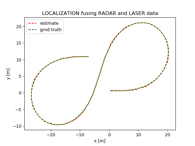
The output is shown in animation in the top figure where blue and red triangles denote noisy measurements of the car obtained from the RADAR and LASER respectively. The estimated pose obtained by fusing these two sensor information using EKF is shown as green dots. Finally estimated path is compared with ground truth data in the figure above.
EKF-SLAM using UTIAS dataset
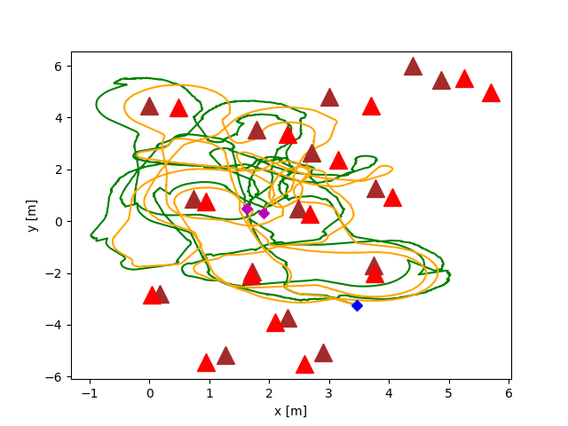
The objective of this project is to localize a mobile robot moving in an unknown environment and also localize the landmarks in the environment. We have used EKF-filtering technique for the localization of the robot itself and the landmarks. The main output of the project is shown in the figure below. The estimated trajectory of the robot is plotted in green and the ground truth of the trajectory is shown in the orange lines. Similarly the estimated locations of the landmarks are plotted in brown triangles and their ground truth locations are plotted in red triangles. The repository can be found here.
Wrapping C for Python Use of IKFast
The repository can be foundhere.
ROS packages for using Realsense and Aruco
The repository can be found here.
Pose Estimation Aruco-Marker in ROS
The repository can be found here.
Robotics Lecture Notes
The repository can be found here.