PID controller experiment: Controlling speed of a turntable

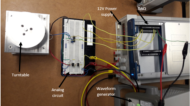
In this page, I will post results that I found while designing a PID controller for a single-input-single-out (SISO) dynamic system. Basically the objective of this experiment was to implementing an analog circuit to communicate a turntable and controlling its speed through a digitally implemented PID controller. The interface between the digital controller and analog circuit is made through a data acquisition system (DAQ) from Texas Instruments. You can see the setup of the experiment below.

The circuit diagram of the above physical circuit is as below.

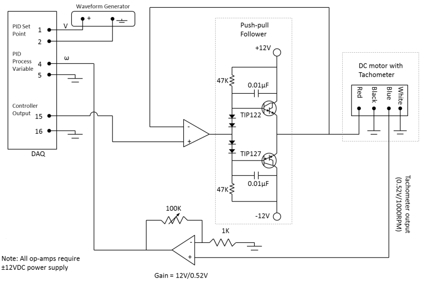
The turntable is controlled by a DC motor with a tachometer. The DC motor rotates at 1000 RPM when connected to a 12V input signal with no-load condition. On the other hand, motor’s speed is measured through the tachometer which produces 0.52V signal for 1000 RPM shaft speed. Therefore, the tachometer output voltage needs to be amplified with a gain ratio of 12V/0.52V to infer the actual input voltage to the DC motor. This has precisely been implemented in the feedback loop amplifier.

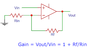
In order to achieve the gain=12V/0.52V in the feedback loop, we need to set the resistance of the potentiometer to 23.3K-Ohm. We calculated the potentiometer resistance value by following the working principle of non-inverting operational-amplifier (Op-Amp) as shown in the figure below.

Deriving Transfer Function of The system

In order to perform theoretical analysis, we need to derive transfer function (TF) of the system. To derive the TF of the whole system, we need to first have the block diagram of the system incorporating the feedback PID loop. The figure below show the block diagram of the whole system with specified blocks representing relevant components. 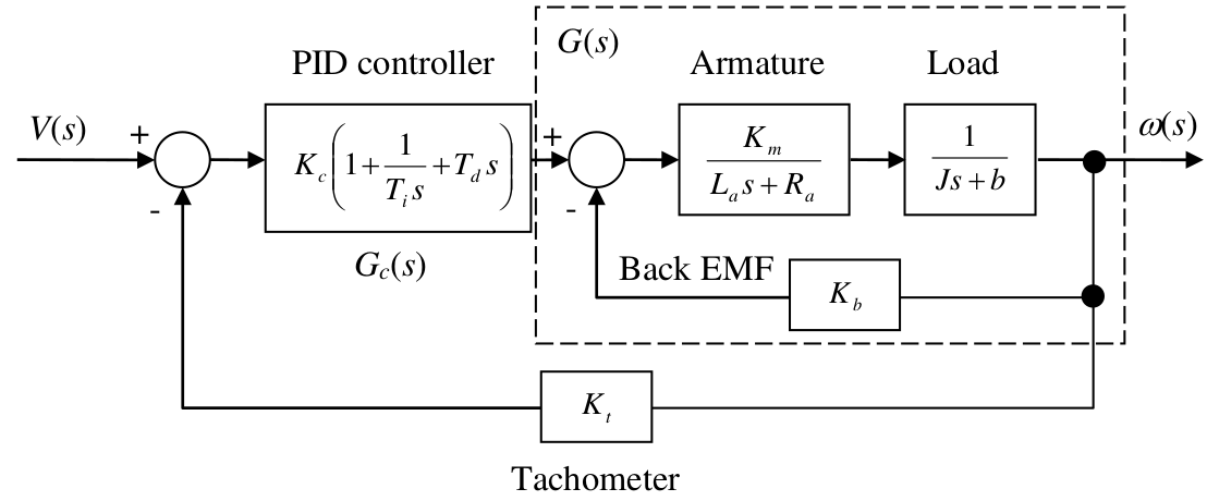Following the block diagram, we write

\(\left(V(s) - K_t\omega(s)\right)G(s)G_c(s) = \omega(s)\) \(\implies T(s) = \frac{\omega(s)}{V(s)}=\frac{G(s)G_c(s)}{1+K_tG(s)G_c(s)}\)

where,

\[G(s) = \frac{K_m}{(L_as+R_a)(Js+b)+K_bK_m}\approx\frac{K_m}{R_a(Js+b)+K_bK_m}\]

\(G_c(s) = K_c(1+\frac{1}{T_is}+T_ds) \implies\) controller transfer function

We assume the parameters associated to DC motor, tachometer and load are as follows

\[K_m = 16.2 OZ-IN/A, R_a = 11.5 \Omega, L_a = 0, J = 2.5 OZ-IN^2\] \[b = 0, K_b = 12V/KRPM, K_t = 12V/KRPM\]

Note: since \(K_b\) and \(K_t\) are given as KRPM, the integration time \((T_i)\) and the derivative time \((T_d)\) are in minutes.

Then from the transfer function derivation, we can find the frequency response i n Laplace domain as,

\[\omega(s) = V(s)T(s)\]

Performing inverse Laplace transform we get the frequency response in time domain as

\[\omega(t) = \mathcal{L}^{-1}(V(s)T(s))\]

Controlling the System using LABVIEW Software

Notice from the physical system setup and/or circuit diagram that the input signal (set point) is connected to the first input channel (port 1 and 2) of the DAQ and process variable (\(\omega\)) is connected to the second input channel (port 4 and 5) of the DAQ. Also the controlling signal is connected to the output channel (port 15 and 16) of the DAQ. This indicates that, if we want to write a software (PID controller) in LABVIEW, we have access to the desired input signal and output from the system through the input channels of the DAQ. Further, output of the PID-controller can be fed into the system through the output channel of the DAQ.

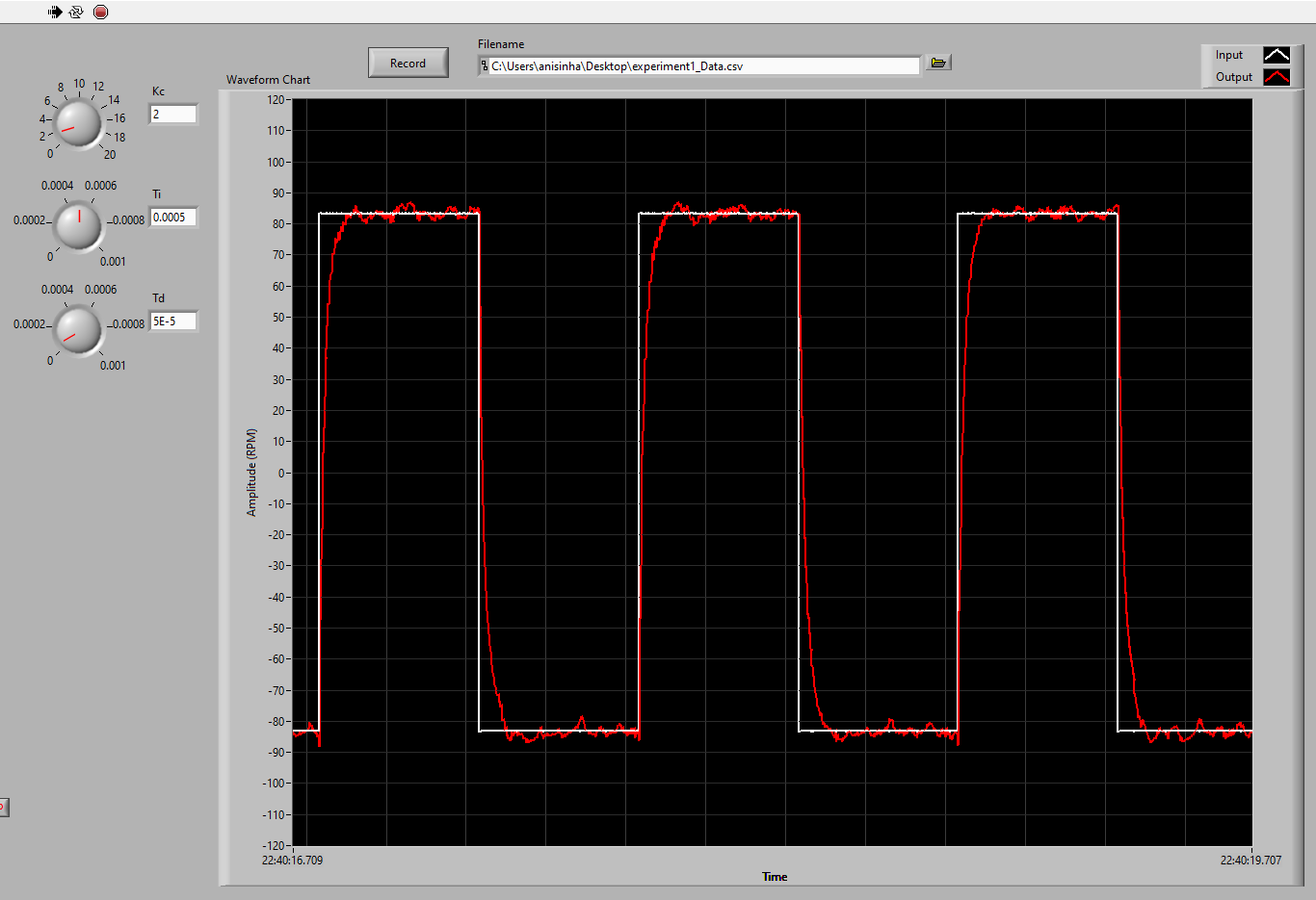
The waveform generator sends 1V signal to the DAQ. For that, the ideal rotational speed of the motor would be \((1000/12)*1=83.3RPM\) RPM. The PID controller generates right amount of control input so that the system’s actual response can match the desired response (in this case 83.3 RPM back and forth).

In this post I am not going to show you how to write a software in LABVIEW, instead, we will adjust the parameters of the PID to a custom made PID controller written in LABVIEW. Figure below shows the screen shot of the input and output responses of the turntable rotational speed while the control parameters are set to \(K_c=1, T_i=5e-4 min, T_d=5e-5 min\) in the application written in LABVIEW. The application also allow us to recorded and write the system input and output responses in a .csv file to be for theoretical analysis. The recorded data for this experiment can be found here.

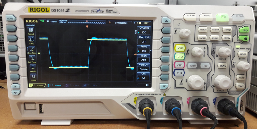
We can also see these signals, in an oscilloscope by connecting the input and output of the system to channel 1 and 2 of the scope as shown below.

Visualize the Recorded Data

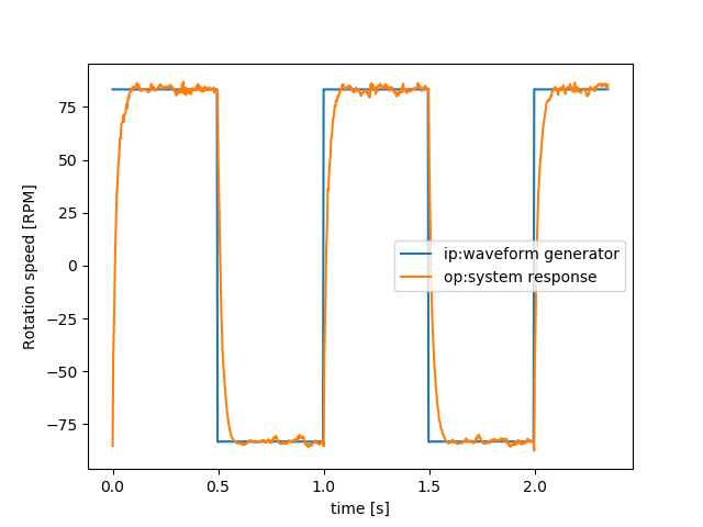
As I have already mentioned that the LABVIEW app for controlling the system has the feature to record the input and output responses of the system in a .csv file, now I will provide a simple python code to read and visualize the recorded data.

import csv
import matplotlib.pyplot as plt

time_arr, ip_arr, op_arr = [], [], []
count = 0
with open("experiment_1/experiment1_Processed_Data.csv") as csv_file:
    csv_reader = csv.reader(csv_file, delimiter=",")
    line_count = 0
    for row in csv_reader:
    	if count >= 25:
    		if count == 25:
    			time_offset = float(row[0])
    		time_arr.append(float(row[0])-time_offset)
    		ip_arr.append(float(row[1]))
    		op_arr.append(float(row[2]))
    	count += 1
    	if count == 800:
        	break
plt.plot(time_arr, ip_arr, label="ip:waveform generator")
plt.plot(time_arr, op_arr, label="op:system response")
plt.xlabel("time [s]")
plt.ylabel("Rotation speed [RPM]")
plt.legend(loc="best")
# plt.grid()
plt.show()

After running the above script in python, we can visualize the data as in the figure below.