Control Project
PID controller experiment
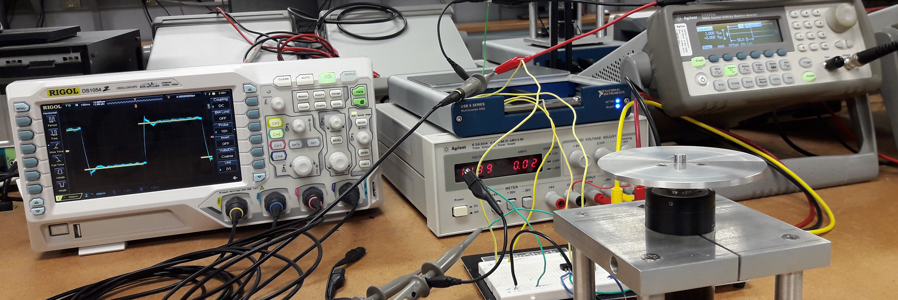
We describe here the effectiveness of PID controller for a single-input-single-output (SISO) system using experiment. The objective of this experiment was to implementing an analog circuit to communicate a turntable and controlling its speed through a digitally implemented PID controller. The interface between the digital controller and analog circuit is made through a data acquisition system (DAQ) from Texas Instruments. You can see the setup of the experiment below.
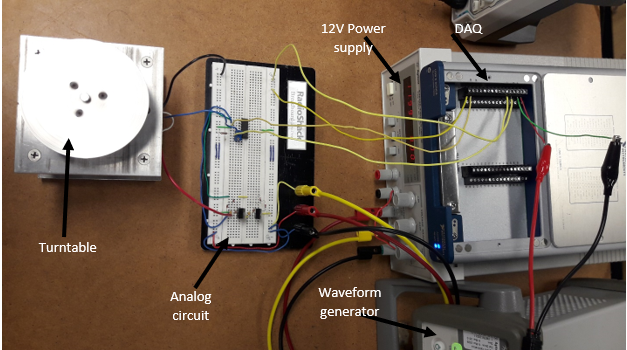
The circuit diagram of the above physical circuit is as below.
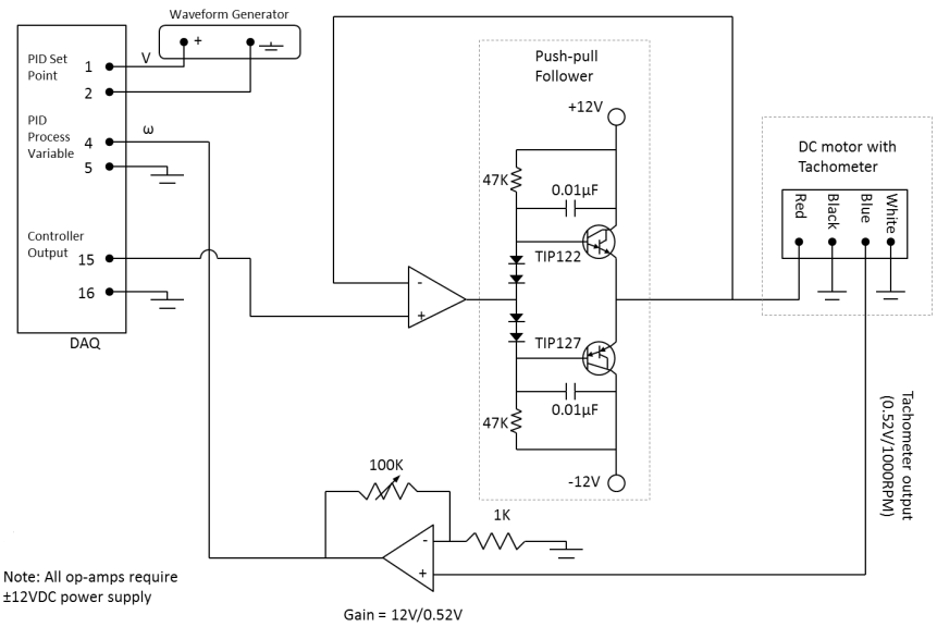
The turntable is controlled by a DC motor with a tachometer. The DC motor rotates at 1000 RPM when connected to a 12V input signal with no-load condition. On the other hand, motor’s speed is measured through the tachometer which produces 0.52V signal for 1000 RPM shaft speed. Therefore, the tachometer output voltage needs to be amplified with a gain ratio of 12V/0.52V to infer the actual input voltage to the DC motor. This has precisely been implemented in the feedback loop amplifier.
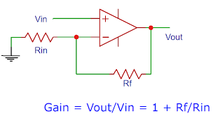
In order to achieve the gain=12V/0.52V in the feedback loop, we need to set the resistance of the potentiometer
to 23.3K-Ohm. We calculated the potentiometer resistance value by following the working principle of non-inverting operational-amplifier (Op-Amp) as shown in the figure below.
Deriving Transfer Function of The system
In order to perform theoretical analysis, we need to derive transfer function (TF) of the system. To derive the TF of the whole system, we need to first have the block diagram of the system incorporating the feedback PID loop. The figure below show the block diagram of the whole system with specified blocks representing relevant components.
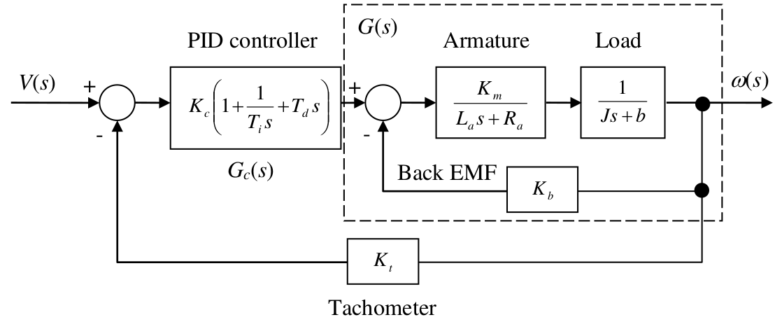 Following the block diagram, we write
\(\left(V(s) - K_t\omega(s)\right)G(s)G_c(s) = \omega(s)\) \(\implies T(s) = \frac{\omega(s)}{V(s)}=\frac{G(s)G_c(s)}{1+K_tG(s)G_c(s)}\)
where,
\[G(s) = \frac{K_m}{(L_as+R_a)(Js+b)+K_bK_m}\approx\frac{K_m}{R_a(Js+b)+K_bK_m}\]\(G_c(s) = K_c(1+\frac{1}{T_is}+T_ds) \implies\) controller transfer function
We assume the parameters associated to DC motor, tachometer and load are as follows
\[K_m = 16.2 OZ-IN/A, R_a = 11.5 \Omega, L_a = 0, J = 2.5 OZ-IN^2\] \[b = 0, K_b = 12V/KRPM, K_t = 12V/KRPM\]Note: since \(K_b\) and \(K_t\) are given as KRPM, the integration time \((T_i)\) and the derivative time \((T_d)\) are in minutes.
Then from the transfer function derivation, we can find the frequency response i n Laplace domain as,
\[\omega(s) = V(s)T(s)\]Performing inverse Laplace transform we get the frequency response in time domain as
\[\omega(t) = \mathcal{L}^{-1}(V(s)T(s))\]Controlling the System using LABVIEW Software
Notice from the physical system setup and/or circuit diagram that the input signal (set point) is connected to the first input channel (port 1 and 2) of the DAQ and process variable (\(\omega\)) is connected to the second input channel (port 4 and 5) of the DAQ. Also the controlling signal is connected to the output channel (port 15 and 16) of the DAQ. This indicates that, if we want to write a software (PID controller) in LABVIEW, we have access to the desired input signal and output from the system through the input channels of the DAQ. Further, output of the PID-controller can be fed into the system through the output channel of the DAQ.
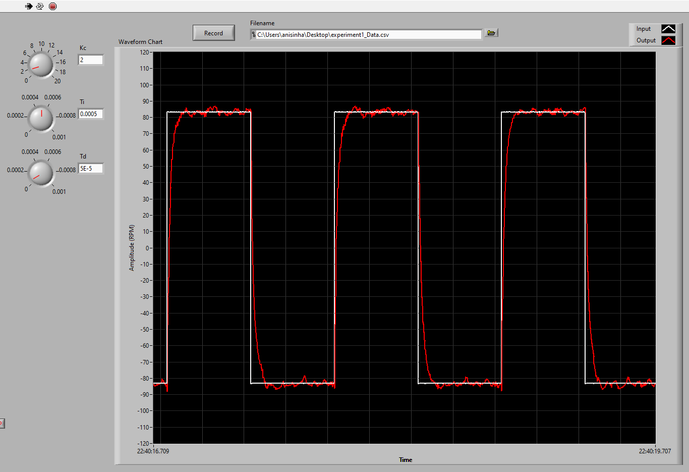
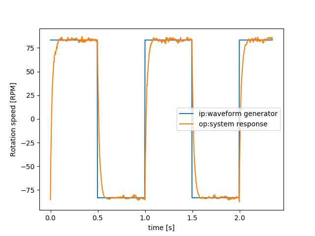
The waveform generator sends 1V signal to the DAQ. For that, the ideal rotational speed of the motor would be \((1000/12)*1=83.3RPM\) RPM. The PID controller generates right amount of control input so that the system’s actual response can match the desired response (in this case 83.3 RPM back and forth).
In this post I am not going to show you how to write a software in LABVIEW, instead, we will adjust the parameters of the PID to a custom made PID controller written in LABVIEW.
Figure below shows the screen shot of the input and output responses of the turntable rotational speed while the control parameters are set to \(K_c=1, T_i=5e-4 min, T_d=5e-5 min\) in the application written in LABVIEW. The application also allow us to recorded and write the system input and output responses in a .csv file to be for theoretical analysis. The recorded data for this experiment can be found here.
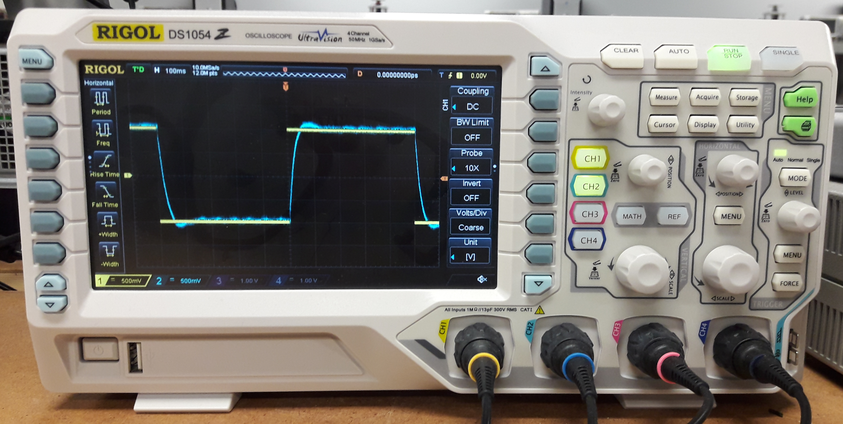
We can also see these signals, in an oscilloscope by connecting the input and output of the system to channel 1 and 2 of the scope as shown below.
Visualize the Recorded Data
As I have already mentioned that the LABVIEW app for controlling the system has the feature to record the input and output responses of the system in a .csv file, now I will provide a simple python code to read and visualize the recorded data.
import csv
import matplotlib.pyplot as plt

time_arr, ip_arr, op_arr = [], [], []
count = 0
with open("experiment_1/experiment1_Processed_Data.csv") as csv_file:
    csv_reader = csv.reader(csv_file, delimiter=",")
    line_count = 0
    for row in csv_reader:
    	if count >= 25:
    		if count == 25:
    			time_offset = float(row[0])
    		time_arr.append(float(row[0])-time_offset)
    		ip_arr.append(float(row[1]))
    		op_arr.append(float(row[2]))
    	count += 1
    	if count == 800:
        	break
plt.plot(time_arr, ip_arr, label="ip:waveform generator")
plt.plot(time_arr, op_arr, label="op:system response")
plt.xlabel("time [s]")
plt.ylabel("Rotation speed [RPM]")
plt.legend(loc="best")
# plt.grid()
plt.show()
After running the above script in python, we can visualize the data as in the figure below.
In this post I will show some theoretical analysis of the PID controller that we have designed in my previous post. After going through this post one will be able to under stand how to derived transfer function of a PID controller, what are the different characteristics of step input response and how are they defined. Finally we will use the data that we have collected in previous postduring the experiment to simulate a PID controller and analyze its step response.
Transfer function of a PID controller
A PID controller block, takes the error signal as input and generates control output signal. In time domain if we define control input as \(u(t)\) and error signal as \(e(t)\), then based on the definition of PID controller, we write
\[u(t) = K_Pe(t) + K_I\int e(t) + K_D \dot{e}(t)\]Taking the Laplace transform we get,
\[U(s) = (K_P + K_I/s + K_Ds)E(s)\]Therefore transfer function of the PID block is obtained as,
\[T(s) = \frac{U(s)}{E(s)} = K_P + \frac{K_I}{s} + K_Ds\]In some applications, it is beneficial to express \(K_I = K_P/T_i\) and \(K_D = K_PT_d\), where \(T_i\) and \(T_d\) are integration and derivative time horizons. This is exactly what we did in PID experiment post to derive the transfer function. In this case, the transfer function of PID controller block would look like as,
\[T(s) = \frac{U(s)}{E(s)} = K_P(1 + \frac{1}{T_is} + T_ds)\]Characteristic of Step Response
There are three main characteristics of the step response.
- Rise time
- Settling time
- Percentage of Overshoot
Rise time \((T_r)\): The time that the response signal would take to reach to 90% from 10% of the steady-state response.
Settling time \((T_s)\): The time that the response signal would take to settle within 2% error relative to the steady-state response.
Percentage of Overshoot: Percentage difference between the maximum peak of the response and steady state response, relative to the steady state response.
Simulated response of turntable
We are now ready to simulate the response of the same PID turn-table experiment for a unit step input. After that we will report the step response characteristics for the simulated system.
From out experiment we found that, the PID controller parameters are \(K_P = 2, T_d = 5e-4 min, T_i = 5e-5 min\). We will be using these paameters to implement the controller. The other system parameters are given in PID turn-table experiment post and will be used them in SI unit form in the simulation.
The python script for simulating the system response with PID controller is given below.
from mpmath import *
import matplotlib.pyplot as plt

def fp(p):
    # Define the given parameters
    Ra = 11.5
    Kb = 12*60/1000                      # convert to V/RPS
    Kt = 12*60/1000                      # convert to V/RPS
    Km = 16.2*0.02835*9.81*0.0254        # convert FPS to SI unit
    J = 2.5*0.02835*9.81*(0.0254**2)     # convert FPS to SI unit
    b = 0
    Kc = 1
    Ti = 0.0005*60                       # convert minute to second
    Td = 0.00005*60                      # convert minute to second

    G = Km/(Ra*(J*p+b)+Kb*Km)            # TF of load
    Gc = Kc*(1 + 1/(Ti*p) + Td*p)        # TF of PID controller
    # Gc = Kc*(1 + Td*p)
    # Gc = Kc
    return Gc*G/(p*(1+Kt*Gc*G))          # TF of the whole system

def step_info(resp, t, resp_final):
	# Find the index for 10% and 90% of total response
	tol = 1e-1
	tl_ind, th_ind, ts_ind, tp = 0, 0, 0, 0
	vl, vh, vs_l, vs_h = 0.10*resp_final, 0.90*resp_final, 0.98*resp_final, 1.02*resp_final
	peak_val = 0
	for ind, val in enumerate(resp):
		# print(ind, val, abs(val-vs), abs(val-resp_final))
		if abs(val-vl) < tol:
			tl_ind = ind
		if abs(val-vh) < tol:
			th_ind = ind
		if ts_ind != 0:
			if vs_l > val or vs_h < val:
				ts_ind = 0
		if vs_l < val and vs_h > val and ts_ind == 0:
			ts_ind = ind
		if val > peak_val:
			peak_val = val
	print("Rise time: %1.3f sec"%(t[th_ind]-t[tl_ind]))
	print("Settling time: %1.3f sec"%t[ts_ind])
	print("Overshoot: %2.3f percent"%((peak_val-resp_final)*100/resp_final))
	return tl_ind, th_ind, ts_ind

mp.dps = 5; mp.pretty = True

# Set point
set_pt = 1000/12

# Generate time vector
tm = [0.0001*tm for tm in range(1, 5000)]

# Multiply the output with 60 to convert RPS to RPM
omega_res = [60*invertlaplace(fp,tt,method='talbot') for tt in tm] # RPM

# Call step_info
stepInfo = step_info(omega_res, tm, set_pt)

plt.plot(tm, omega_res)
plt.plot([tm[stepInfo[0]], tm[stepInfo[0]]], [0, omega_res[stepInfo[0]]], "C1")
plt.plot([tm[stepInfo[1]], tm[stepInfo[1]]], [0, omega_res[stepInfo[1]]], "C1")
plt.plot([tm[stepInfo[2]], tm[stepInfo[2]]], [0, omega_res[stepInfo[2]]], "C2")
print(omega_res[stepInfo[1]]/2)
plt.text(tm[stepInfo[1]]/2, omega_res[stepInfo[1]]/2, "rise time")
plt.text(tm[stepInfo[2]], omega_res[stepInfo[2]]/2, "setteling time")
plt.xlabel("time [s]")
plt.ylabel(r"$\omega$(t) [RPM]")
plt.title("Step response for PID controller")
plt.grid()
plt.show()
The simulated response of the turntable with PID controller is found after running the above script is shown below.
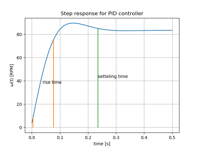
The rise time, settling time and percent of overshoot values are found to be,
Rise time: 0.073 sec
Settling time: 0.235 sec
Overshoot: 7.474 %
LABVIEW application
The figure below shows the basic LABVIEW program that can be used to acquire and send signal to the system for the DAQ connections as per the post on PID experiment post.
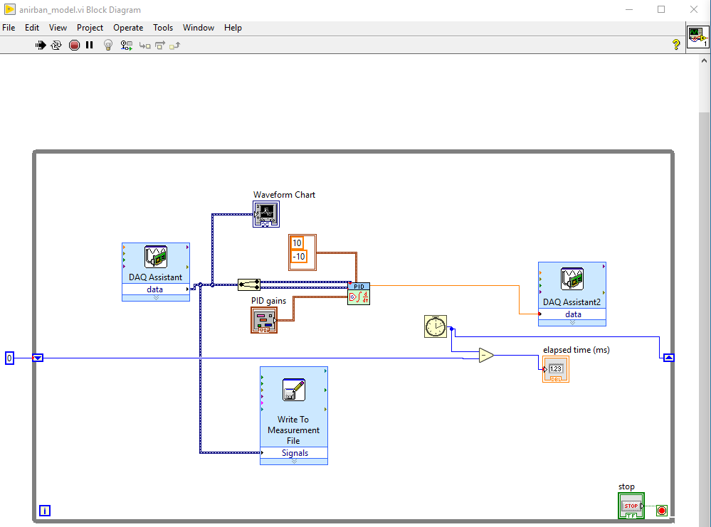
I only used a few number of code blocks to achieve the above and they are
- DAQ Assistant (1 input and 1 output)
- Waveform Chart
- Write to Measurement File
- PID
- Split Signal
- While Loop with Button
- While Shift
- Numeric
- Cluster
- Create Control
- Comparison
- Elapsed Time
